I’m starting 2021 with one of the essential New Year’s resolutions: Practice more complex SQL queries. If you’re on the same boat, join me to explore 3 useful SQL features with Google BigQuery.

You’ll learn how to:

1. Create tables with date partitions
2. Aggregate over a group of rows with (analytic) window functions
3. Break down complex queries using WITH clause

Depending on your background, these might seem like basic features that appeared in other relational databases or they may appear exotic. Either way, I have included detailed examples and approach on how I tackled each query. So let’s hop into something comfy and dive right in!

Before you begin

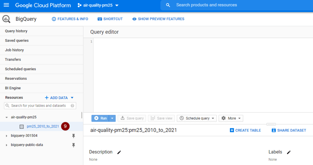
In Google BigQuery, you will need to be aware of the following hierarchy: Project – Dataset – Tables/ Views

• A project organises all resources (e.g. data, storage, compute engine, etc.) to be used. A project can include one or multiple datasets.
• A dataset is a container to organise and control access to tables and views. A dataset can include one or many tables and/or views.

Before analysing any data, we have to create a project and a dataset. Here is how to do it in less than 3 minutes.  

Create a project

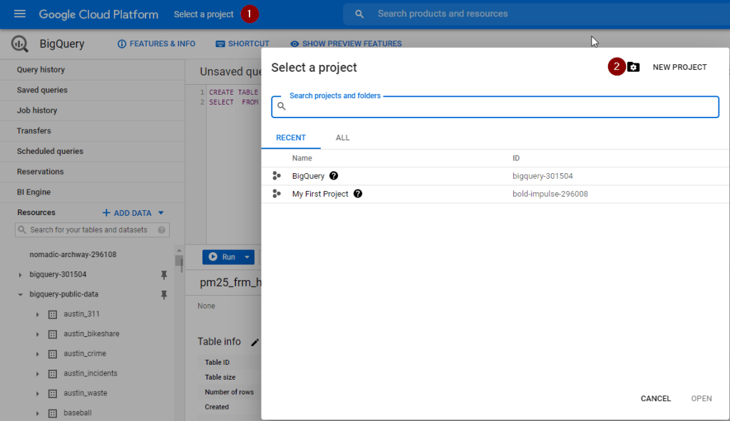
Click on Select a project and select New Project

Upon seeing the below screen, specify the project name of your choice and click Create.

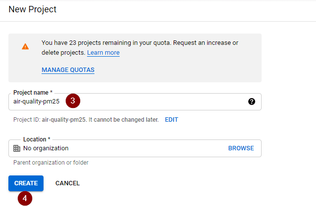
It will take around 10-20 seconds for project creation to complete. Notification regarding the status of completion can be viewed by clicking on the Bell icon located at the top right corner of the screen.

Create a dataset

Next, you will create a dataset to store your new tables.

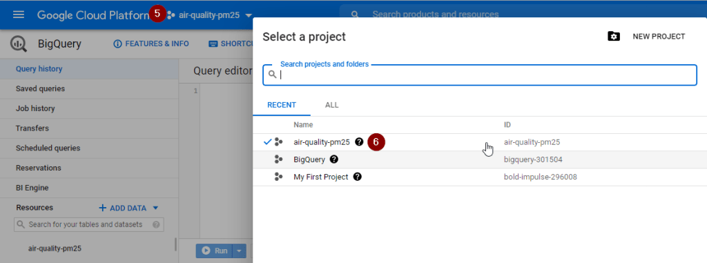
Check the project name shown at the top menu next to Google Cloud Platform. If that is not newly created project, click Select a project and switch to the correct one.

Select the project name, then click Create Dataset

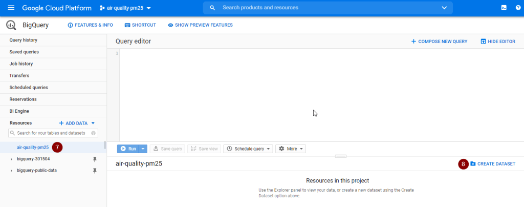
Upon seeing the new dataset under the new project (as shown below), you are all set and ready to get started.

Create tables with date partitions

Goal

Create a new table including all daily average levels of PM2.5 particles in the air from 2010 onwards.

Also, in the new table, include a new column to indicate the air quality category based on PM2.5 levels.

PM2.5 Level (µg/m3)	Air Quality Category
Less than 12.5	Good
12.5-25	Fair
25-50	Poor
50-150	Very Poor
More than 150	Extremely Poor

PM2.5 particles are a common air pollutant usually found in smoke. They are small enough for human to breathe deeply into our lungs or enter our bloodstream. People who are sensitive to air pollution might experience chest tightness, difficulty breathing, aggravated asthma or irregular heartbeat when PM2.5 levels are high.

From Environment Protection Authority Victoria, Australia

Approach

1. Create a new permanent table to isolate PM2.5 levels from 2010 onwards for subsequent queries, thus skipping all historical records before 2020 (assuming we are only interested in 2010 onwards).
2. Only select necessary columns from the original dataset to avoid wasting time and cost on scanning through irrelevant columns.
3. Bind the year of date_local column as a partition to divide the new table into smaller partitions to improve query performance and control costs by reducing the number of bytes read by a query.
4. Leverage CASE statement to create a new column to map air quality category against arithmetic_mean

Query

#standardSQL
CREATE OR REPLACE TABLE
  pm25.partition_by_day
  #Bind the year of date_local as a partition
PARTITION BY
  DATE_TRUNC(date_local, year) OPTIONS (description = "Daily PM2.5 from 2010 onwards partitioned by date") AS

#Only select necessary columns
SELECT
 state_code, county_code, site_num, poc, sample_duration, event_type, latitude,
 longitude, date_local, units_of_measure, arithmetic_mean, state_name,   county_name,

#Include a new column to specify air quality category with CASE statement
  CASE
    WHEN arithmetic_mean < 12.5 THEN "Good"
    WHEN arithmetic_mean >= 12.5 AND arithmetic_mean < 25 THEN "Fair"
    WHEN arithmetic_mean >= 25 AND arithmetic_mean <50 THEN "Poor"
    WHEN arithmetic_mean >=50 AND arithmetic_mean <=150 THEN "Very Poor"
    WHEN arithmetic_mean > 150 THEN "Extremely Poor"
END
  AS air_quality_category
FROM
  `bigquery-public-data.epa_historical_air_quality.pm25_frm_daily_summary`
WHERE
  date_local > "2010-1-1"
  AND sample_duration = "24 HOUR"
  AND poc = 1
  AND (event_type = "Excluded" OR event_type = "None");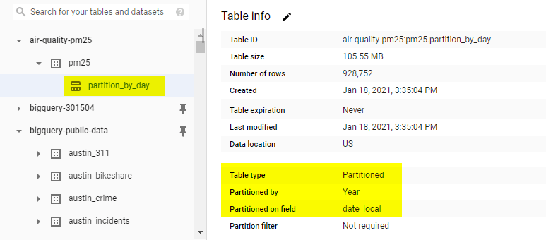

Ten-second takeaway

If you only care about records for a specific period (e.g. last year, within the last 7 days), creating a date-partitioned table will allow us to completely ignore scanning records in certain partitions if they are irrelevant to our query, thus saving query time and costs.

Aggregate over a group of rows with window functions

Goal

For each state, to identify which county, the exact location and date that had the highest daily level of PM2.5 particles in 2019

Approach

1. Look at all 2019 readings, rank all arithmetic_mean over groups of state records in descending order
2. Include the state_name, county_name, latitude, longitude, date_local together with those max levels per state identified above
3. Only select records with the highest arithmetic_mean (i.e. rank = 1)

Query

#standardSQL
# Rank all PM2.5 levels by state
WITH
  rank_by_state AS (
  SELECT
    state_name,
 county_name,
 latitude,
 longitude,
 date_local,
 arithmetic_mean,
    RANK() OVER (PARTITION BY state_code ORDER BY arithmetic_mean DESC) AS rank
  FROM
    `air-quality-pm25.pm25.partition_by_day`
  WHERE
    date_local >= "2018-01-01"
 AND date_local <= "2018-12-31")

#Select only the highest PM2.5 level
SELECT
  state_name,
 county_name,
 latitude,
 longitude,
 date_local,
 arithmetic_mean AS daily_pm_25
FROM
  rank_by_state
WHERE
  rank = 1
ORDER BY daily_pm_25 DESC;

Remember those SQL tricky interview questions to find the second highest, third highest and so on? This query also works well since you can easily substitute the WHERE clause for rank = 1 with 2, 3 and so on.

Ten-second takeaway

To evaluate aggregate values over a group of rows (i.e. highest value by state/ month/ year), opt for (analytic) window functions instead of using expensive self-JOINs.

Break down complex queries using WITH clause

Example 1

Goal

In 2019, which counties have at least 5 days with poor air quality (i.e. average daily quantity of PM2.5 reached 25 micrograms or above)? For each county, how many days of poor air quality in total?

Approach

1. Calculate the daily average of PM2.5 level for each county in 2019
2. For each county, count the number of days where PM2.5 reached 25 micrograms or above
3. Include only counties with at least 5 days, together with the number of days where PM2.5 reached 25 micrograms or above. Sort by number of days in descending order to highlight county and state having the most days with poor air quality

Query

#standardSQL
WITH
  daily_pm25 AS (

#Calculate the daily average of PM2.5 level for each county in 2019
  SELECT
    state_name,
 county_name,
 date_local,
 AVG( arithmetic_mean) AS average_pm25
  FROM
    `air-quality-pm25.pm25.partition_by_day`
  WHERE
    date_local >= "2019-01-01"
 AND date_local <= "2019-12-30"
  GROUP BY
    state_name,
 county_name,
 date_local)

#Count the number of days where PM2.5 reached 25 micrograme or above
SELECT
  state_name,
 county_name,
 COUNT(date_local) AS number_of_days
FROM
  daily_pm25
WHERE
  average_pm25 >= 25
GROUP BY
  state_name,
 county_name
  
#Include only counties with at least 5 days of poor air quality
HAVING
  number_of_days >= 5
ORDER BY
  number_of_days DESC;

Ten-second takeaway

To solve a complex query, use the WITH clause (a.k.a. Common Expression Table) to break apart the complex question into many smaller steps and tables instead of trying to write one massive combined SQL statement.

Bonus tip: If the table within the WITH clause can be reused across different queries, consider creating a permanent table to store the query result. In doing so, you can avoid running the same query inside the WITH clause multiple times.

Example 2

Goal

For each state and county, what is the difference between the annual average level of PM2.5 in 2018 and 2019?

Approach

1. For each state and county, calculate the annual average level of PM2.5 in 2018
2. For each state and county, calculate the annual average level of PM2.5 in 2019
3. Combine these 2 results into 1 table and calculate the difference between PM2.5 level between 2018 and 2019. Round the difference to 2 decimal places for easy comparison.

Query

#standardSQL
#Calculate annual average of 2018
WITH
  pm25_2018 AS (
  SELECT
    state_name,
 county_name,
 AVG(arithmetic_mean) AS average_2018
  FROM
    `air-quality-pm25.pm25.partition_by_day`
  WHERE
    date_local >= "2018-01-01"
 AND date_local <="2018-12-31"
  GROUP BY
    state_name,
 county_name
  ORDER BY
    average_2018 DESC),
  
#Calculate annual average of 2019
  pm25_2019 AS (
  SELECT
    state_name,
 county_name,
 AVG(arithmetic_mean) AS average_2019
  FROM
    `air-quality-pm25.pm25.partition_by_day`
  WHERE
    date_local >= "2019-01-01"
 AND date_local <="2019-12-31"
  GROUP BY
    state_name,
 county_name)
  
#Combine both tables and calculate the difference between 2018 and 2019
SELECT
  pm25_2018.state_name,
 pm25_2018.county_name,
 average_2018,
 average_2019,
  ROUND(average_2019 - average_2018,2) AS difference
FROM
  pm25_2018
JOIN
  pm25_2019
USING
  (state_name,
 county_name)
ORDER BY
  difference DESC;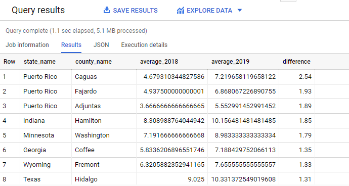

Ten-second takeaway

To make a complex query more readable, use WITH clause to create multiple table expressions, then join the resulting tables.

Wrapping Up

Despite showing you long queries and a brief explanation of my approach, this article covered only a small part of what can be done with Google BigQuery. However, I hope this has provided you with a good starting point for all the insightful queries that you will be writing. Inevitably you will hit a roadblock or get stuck with a difficult SQL question. In such a case, remember to take a deep breath, grab something to drink and start breaking down the big question into smaller chunks like how I did in my approach. You’re almost there and you will conquer it!

With that, thank you for reading and do let me know if you have any feedback. Have a good one!